43 excel pie chart add labels

How to display leader lines in pie chart in Excel? - ExtendOffice To display leader lines in pie chart, you just need to check an option then drag the labels out. 1. Click at the chart, and right click to select Format Data Labels from context menu. 2. In the popping Format Data Labels dialog/pane, check Show Leader Lines in the Label Options section. See screenshot: 3. Close the dialog, now you can see some leader lines appear. If you want to show all leader lines, just drag the labels out of the pie one by one. Inserting Data Label in the Color Legend of a pie chart Re: Inserting Data Label in the Color Legend of a pie chart @SabrinaFr There is no built-in way to do that, but you can use a trick: see Add Percent Values in Pie Chart Legend (Excel 2010)

Office: Display Data Labels in a Pie Chart - Tech-Recipes 3. In the Chart window, choose the Pie chart option from the list on the left. Next, choose the type of pie chart you want on the right side. 4. Once the chart is inserted into the document, you will notice that there are no data labels. To fix this problem, select the chart, click the plus button near the chart's bounding box on the right ...

Excel pie chart add labels

Add a DATA LABEL to ONE POINT on a chart in Excel All the data points will be highlighted. Click again on the single point that you want to add a data label to. Right-click and select ' Add data label '. This is the key step! Right-click again on the data point itself (not the label) and select ' Format data label '. You can now configure the label as required — select the content of ... How to Create Pie Charts in Excel (In Easy Steps) Click the + button on the right side of the chart and click the check box next to Data Labels. 10. Click the paintbrush icon on the right side of the chart and change the color scheme of the pie chart. Result: 11. Right click the pie chart and click Format Data Labels. 12. Check Category Name, uncheck Value, check Percentage and click Center. Add data labels and callouts to charts in Excel 365 - EasyTweaks.com The steps that I will share in this guide apply to Excel 2021 / 2019 / 2016. Step #1: After generating the chart in Excel, right-click anywhere within the chart and select Add labels . Note that you can also select the very handy option of Adding data Callouts.

Excel pie chart add labels. Online Web Development Tutorial Excel Charts - Aesthetic Data Labels Data labels stay in place, even when you switch to a different type of chart. You can also connect the data labels to their data points with leader lines on all charts. Here, we will use a Bubble chart to see the formatting of data labels. excel - How to not display labels in pie chart that are 0% - Stack Overflow Then right click on the labels and choose "Format Data Labels" Check "Value From Cells", choosing the column with the formula and percentage of the Label Options. Under Label Options -> Number -> Category, choose "Custom" Under Format Code, enter the following: 0%;; Result should look like this: (labels selected so you can see there's a blank one) Hide and show chart labels in Excel For example, the following chart has been created: 1. Want to add detailed sales for employees displayed right on the chart do the following:-Click on the chart -> Design -> Add Chart Element -> Data labels -> select the data placement, for example, choose OutSide End: - Revenue data results show after the end of the data column: 2. Show more ... How to Insert Axis Labels In An Excel Chart | Excelchat We will again click on the chart to turn on the Chart Design tab We will go to Chart Design and select Add Chart Element Figure 6 - Insert axis labels in Excel In the drop-down menu, we will click on Axis Titles, and subsequently, select Primary vertical Figure 7 - Edit vertical axis labels in Excel

Excel charts: add title, customize chart axis, legend and data labels ... Click anywhere within your Excel chart, then click the Chart Elements button and check the Axis Titles box. If you want to display the title only for one axis, either horizontal or vertical, click the arrow next to Axis Titles and clear one of the boxes: Click the axis title box on the chart, and type the text. [SOLVED] Pie Chart Data Labels - Excel Help Forum No, the chart tool add-ins only have to be installed on the machine in which you are working to add the labels. I forgot to add another way to customize data labels . . . You can also click inside of the individual data label and then add a reference to a cell. For example, you can click inside of the › how-to-show-percentage-inHow to Show Percentage in Pie Chart in Excel? - GeeksforGeeks Jun 29, 2021 · Select a 2-D pie chart from the drop-down. A pie chart will be built. Select -> Insert -> Doughnut or Pie Chart -> 2-D Pie. Initially, the pie chart will not have any data labels in it. To add data labels, select the chart and then click on the “+” button in the top right corner of the pie chart and check the Data Labels button. How to add axis label to chart in Excel? - ExtendOffice Select the chart that you want to add axis label. 2. Navigate to Chart Tools Layout tab, and then click Axis Titles, see screenshot: 3.

support.microsoft.com › en-us › officeAdd a pie chart - support.microsoft.com To switch to one of these pie charts, click the chart, and then on the Chart Tools Design tab, click Change Chart Type. When the Change Chart Type gallery opens, pick the one you want. See Also. Select data for a chart in Excel. Create a chart in Excel. Add a chart to your document in Word. Add a chart to your PowerPoint presentation Creating Pie Chart and Adding/Formatting Data Labels (Excel) Creating Pie Chart and Adding/Formatting Data Labels (Excel) - YouTube. c# - Add data labels to excel pie chart - Stack Overflow Add data labels to excel pie chart. private void DrawFractionChart (Excel.Worksheet activeSheet, Excel.ChartObjects xlCharts, Excel.Range xRange, Excel.Range yRange) { Excel.ChartObject myChart = (Excel.ChartObject)xlCharts.Add (200, 500, 200, 100); Excel.Chart chartPage = myChart.Chart; Excel.SeriesCollection seriesCollection = chartPage. Multiple data labels (in separate locations on chart) You can do it in a single chart. Create the chart so it has 2 columns of data. At first only the 1 column of data will be displayed. Move that series to the secondary axis. You can now apply different data labels to each series. Attached Files 819208.xlsx‎ (13.8 KB, 264 views) Download Cheers Andy Register To Reply

Excel Charts: Excel Pie Chart With Individual Slice Radius

Microsoft Excel Tutorials: Add Data Labels to a Pie Chart To add the numbers from our E column (the viewing figures), left click on the pie chart itself to select it: The chart is selected when you can see all those blue circles surrounding it. Now right click the chart. You should get the following menu: From the menu, select Add Data Labels. New data labels will then appear on your chart:

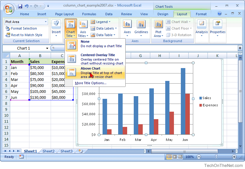
MS Excel 2007: How to Create a Column Chart

Edit titles or data labels in a chart - support.microsoft.com On a chart, click one time or two times on the data label that you want to link to a corresponding worksheet cell. The first click selects the data labels for the whole data series, and the second click selects the individual data label. Right-click the data label, and then click Format Data Label or Format Data Labels.

How to Create Multi-Category Chart in Excel - Excel Board

Adding data labels to a Pie Chart in VBA - Automate Excel Adding data labels to a Pie Chart in VBA - Automate Excel.

Excel charts: Mastering pie charts, bar charts and more | PCWorld

How to Make a Pie Chart in Excel & Add Rich Data Labels to The Chart! Creating and formatting the Pie Chart. 1) Select the data. 2) Go to Insert> Charts> click on the drop-down arrow next to Pie Chart and under 2-D Pie, select the Pie Chart, shown below. 3) Chang the chart title to Breakdown of Errors Made During the Match, by clicking on it and typing the new title.

Share :