41 how to put data labels in excel chart
How to Add Leader Lines in Excel? - GeeksforGeeks Step 2: Go to Insert Tab and select Recommended Charts. A dialogue box name Insert Chart appears. Step 3: Click on All Charts and select Line. Click Ok. Step 4: A line chart is embedded in the worksheet. Step 5: Go to Chart Design Tab and select Add Chart Element . Step 6: Hover on the Data Labels option. Click on More Data Label Options …. how to edit a legend in Excel — storytelling with data How to do it in Excel: Click on your graph, and then in your Excel ribbon, select the "Format" tab next to the "Chart Design" tab. Towards the left hand side of your ribbon, click on the icon of a text box. That will place a blank text box in your Chart Area, which you can move, edit, and format just like a regular text box.
Excel: How To Convert Data Into A Chart/Graph - Rowan University 7: To add axis titles, data labels, legend, trendline, and more, click the graph you just created. A new tab titled "Chart design" should appear. In the upper menu of that tab, you should see a section called "add chart element." 8: In "add chart element," you can customize your graph to your liking . STEP 9: Don't forget to save your work!
How to put data labels in excel chart
How to Make a Pie Chart in Excel (Only Guide You Need) To do this select the More Options from Data labels under the Chart Elements or by selecting the chart right click on to the mouse button and select Format Data Labels. This will open up the Format Data Label option on the right side of your worksheet. Click on the percentage. If you want the value with the percentage click on both and close it. how to create a line chart in Excel — storytelling with data To begin, highlight the data table, including the column headers. To do this, click cell B7 and drag your cursor to C18. Next, navigate to the Insert ribbon and select the line chart icon. (Note that you can also use the Insert menu at the very top, then choose Chart -> Line to achieve a similar result.) How to Create a Dynamic Chart Title in Excel Select chart title in your chart. Go to the formula bar and type =. Select the cell which you want to link with chart title. Hit enter. Related: Combine Cell Link and Text to Create a Dynamic Chart Title Now, let me show you how to combine a cell and a text to create a dynamic chart title.
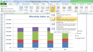
How to put data labels in excel chart. How to Apply a Filter to a Chart in Microsoft Excel Select the data for your chart, not the chart itself. Go to the Home tab, click the Sort & Filter drop-down arrow in the ribbon, and choose "Filter." Click the arrow at the top of the column for the chart data you want to filter. Use the Filter section of the pop-up box to filter by color, condition, or value. How to Add Axis Label to Chart in Excel - Sheetaki Select the chart that you want to add an axis label. Next, head over to the Chart tab. Click on the Axis Titles. Navigate through Primary Horizontal Axis Title > Title Below Axis. An Edit Title dialog box will appear. In this case, we will input "Month" as the horizontal axis label. Next, click OK. Display data point labels outside a pie chart in a paginated report ... Create a pie chart and display the data labels. Open the Properties pane. On the design surface, click on the pie itself to display the Category properties in the Properties pane. Expand the CustomAttributes node. A list of attributes for the pie chart is displayed. Set the PieLabelStyle property to Outside. Set the PieLineColor property to Black. How to: Display and Format Data Labels - DevExpress Add Data Labels to the Chart; Specify the Position of Data Labels; Apply Number Format to Data Labels; Create a Custom Label Entry; Add Data Labels to the Chart. Basic settings that specify the contents, position and appearance of data labels in the chart are defined by the DataLabelOptions object, accessed by the ChartView.DataLabels property ...
How to Find, Highlight, and Label a Data Point in Excel Scatter Plot? By default, the data labels are the y-coordinates. Step 3: Right-click on any of the data labels. A drop-down appears. Click on the Format Data Labels… option. Step 4: Format Data Labels dialogue box appears. Under the Label Options, check the box Value from Cells . Step 5: Data Label Range dialogue-box appears. How to make a quadrant chart using Excel - Basic Excel Tutorial Format data labels. Right-click on any label and select 'Format Data Labels.' Go to the 'Label Options' tab and check the 'Value from cells' option. Select all the names and click OK. Uncheck the 'Y Value' box and under 'Label Position,' select 'Above. 7. Add the Axis titles. Select the chart and go to the 'Design' tab. Choose 'Add Chart ... Modifying Axis Scale Labels (Microsoft Excel) Follow these steps: Create your chart as you normally would. Double-click the axis you want to scale. You should see the Format Axis dialog box. (If double-clicking doesn't work, right-click the axis and choose Format Axis from the resulting Context menu.) Make sure the Number tab is displayed. (See Figure 1.) How To Add a Target Line in Excel (Using Two Different Methods) Use the following steps to add a target line in your Excel spreadsheet by adding a new data series: 1. Open your Excel spreadsheet To add a target line in Excel, first, open the program on your device. Then create a new spreadsheet by clicking "New." You also can open an existing one with the data you want to use for your bar graph. 2.
Excel: How to Create a Bubble Chart with Labels - Statology Step 3: Add Labels. To add labels to the bubble chart, click anywhere on the chart and then click the green plus "+" sign in the top right corner. Then click the arrow next to Data Labels and then click More Options in the dropdown menu: In the panel that appears on the right side of the screen, check the box next to Value From Cells within ... How Insert Stiff Diagram in Excel | Microsoft Excel Tips | Excel ... Step 5: Now go to Insert-> Charts-> Insert Scatter. Step 6: Now assign the data labels by the values in the first table. Select the blue dots by click-> right click-> format data labels. Step 7: Select value from cells and then provide the range of cation names. Step 8: Format Data Labels-> Size and Properties-> Text Direction-> Rotate 90 ... How To Create Labels In Excel moonmilkreview Create labels from excel in a word document. All words describing the values (numbers) are called labels. Excel labels, values, and formulas. Click finish & merge in the finish group on the mailings tab. Select mailings > write & insert fields > update labels. The next time you open the document, word will ask you whether you want to merge the ... Custom Chart Data Labels In Excel With Formulas Follow the steps below to create the custom data labels. Select the chart label you want to change. In the formula-bar hit = (equals), select the cell reference containing your chart label's data. In this case, the first label is in cell E2. Finally, repeat for all your chart laebls.
32 Data Label Excel - Labels Design Ideas 2020
How to Print Labels from Excel - Lifewire Choose Start Mail Merge > Labels . Choose the brand in the Label Vendors box and then choose the product number, which is listed on the label package. You can also select New Label if you want to enter custom label dimensions. Click OK when you are ready to proceed. Connect the Worksheet to the Labels
Charts in Excel - Easy Excel Tutorial
Step-by-Step Guide on How to Make a Chart in Excel (And Tips) Here's a list of the step-by-step process for how to make a chart in Excel: 1. Create your spreadsheet. First, open the spreadsheet with the relevant data you want to put in the chart or graph. If you don't have an existing document, you can create a new spreadsheet and manually input the data.
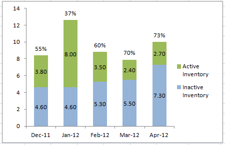
How-to Put Percentage Labels on Top of a Stacked Column Chart - Excel Dashboard Templates
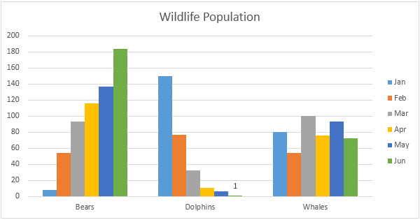
How to Add Labels to Scatterplot Points in Excel - Statology Next, click anywhere on the chart until a green plus (+) sign appears in the top right corner. Then click Data Labels, then click More Options… In the Format Data Labels window that appears on the right of the screen, uncheck the box next to Y Value and check the box next to Value From Cells.

E-xcel Tuts: Add Data Labels to Excel Charts
How to Create and Customize a Treemap Chart in Microsoft Excel Either right-click the chart and pick "Format Chart Area" or double-click the chart to open the sidebar. On Windows, you'll see two handy buttons on the right of your chart when you select it. With these, you can add, remove, and reposition Chart Elements. And you can pick a style or color scheme with the Chart Styles button.
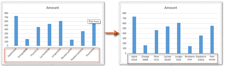
How to wrap X axis labels in a chart in Excel?
How to add secondary axis in Excel (2 easy ways) - ExcelDemy 1) In this way, at first, select all the data, or select a cell in the data. You see, we have selected a cell within the data that we shall use to make the chart. 2) Now go to Insert tab => click on the Recommended Charts command in the Charts window or click on the little arrow icon on the bottom right corner of the window.
30 What Is Data Label In Excel - Labels Design Ideas 2020
Chart.ApplyDataLabels method (Excel) | Microsoft Docs ApplyDataLabels ( Type, LegendKey, AutoText, HasLeaderLines, ShowSeriesName, ShowCategoryName, ShowValue, ShowPercentage, ShowBubbleSize, Separator) expression A variable that represents a Chart object. Parameters Example This example applies category labels to series one on Chart1. VB Copy Charts ("Chart1").SeriesCollection (1).

How to Make Charts and Graphs in Excel | Smartsheet
How To Show Two Sets of Data on One Graph in Excel To do so, click and drag your mouse across all the data you want, including the names of the columns and rows. You can check that you selected the data by looking for the cells to be gray instead of white. 3. Click the "Insert" tab and then look at the "Recommended Charts" in the charts group
charts - Showing percentages above bars on Excel column graph - Stack Overflow
Pivot Chart Data Label Formatting Question - Microsoft Tech Community Hi, I have a pivot chart. I format the data labels, for example make the text larger or turn it. Every time I refresh the data the data label formatting reverts to the default. I have gone to the Pivot Chart options and made sure the Preserve cell formatting option is checked. How to I get around...

Creating Pie Chart and Adding/Formatting Data Labels (Excel) - YouTube
【How-to】How to make a waterfall chart in excel - Howto.org Insert a waterfall chart in Excel. Start with selecting your data. Include the data label in your selection for it to be recognized automatically by Excel. Activate the Insert tab in the Ribbon and click on the Waterfall Chart icon to see the chart types under category. Click the Waterfall chart to create your chart.
How to Add Data Labels in Excel - Excelchat | Excelchat
How to Create a Dynamic Chart Title in Excel Select chart title in your chart. Go to the formula bar and type =. Select the cell which you want to link with chart title. Hit enter. Related: Combine Cell Link and Text to Create a Dynamic Chart Title Now, let me show you how to combine a cell and a text to create a dynamic chart title.

Mapping relationships between people using interactive network chart » Chandoo.org - Learn Excel ...
how to create a line chart in Excel — storytelling with data To begin, highlight the data table, including the column headers. To do this, click cell B7 and drag your cursor to C18. Next, navigate to the Insert ribbon and select the line chart icon. (Note that you can also use the Insert menu at the very top, then choose Chart -> Line to achieve a similar result.)
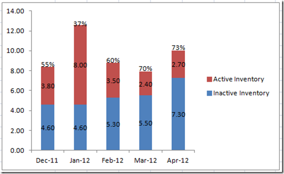
How-to Put Percentage Labels on Top of a Stacked Column Chart - Excel Dashboard Templates
How to Make a Pie Chart in Excel (Only Guide You Need) To do this select the More Options from Data labels under the Chart Elements or by selecting the chart right click on to the mouse button and select Format Data Labels. This will open up the Format Data Label option on the right side of your worksheet. Click on the percentage. If you want the value with the percentage click on both and close it.

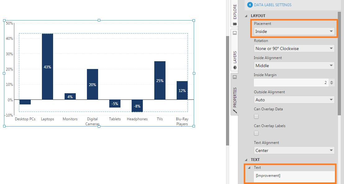
Show Trend Arrows in Excel Chart Data Labels

Automatically update data labels on Excel chart (Excel 2016) - Stack Overflow

Chart Data Labels in PowerPoint 2011 for Mac
How-to Add Custom Labels that Dynamically Change in Excel Charts - Excel Dashboard Templates
Post a Comment for "41 how to put data labels in excel chart"